New additions as of OUwie 2.1
Jeremy M. Beaulieu and Brian C. O’Meara
Source:vignettes/OUwie_2.1_adds.Rmd
OUwie_2.1_adds.RmdIt’s been quite a while since we’ve done any active development of
OUwie. It was recently brought to our attention that the
likelihoods between OUwie and ouch are not the
same when the model assumes different OU means (what we refer to here as
“OUM”). We would like to thank and credit Clay Cressler for working
through our code to identify the specific causes. In doing so, we have
taken this opportunity to release a new version of OUwie
that provides cleaner output and a number of new capabilities. Some of
these new functions were implemented at the request of users, for our
own research, and as part of tutorials for various workshops.
Bug fixes and deprecated functions
The differences between OUwie and ouch were
traced to two issues. There first being a bug in the most recent version
of the weight matrix generation code. For some reason, while looping
over the different regimes, the function was not resetting the regime to
the regime at the root, and the calculation for the weights for the root
regime was missing a
term. These are now fixed, and fortunately does not cause any detectable
effect on the likelihood, though it does have a slight impact on the
estimates of the regime optima.
The second issue is significant and has to do with the way
OUwie and ouch construct the
variance-covariance matrix when assuming stationarity at the root. In
Beaulieu et al. (2012), we expanded upon equation A5 in Butler and King
(2004), which assumed that the root optima was estimated. We found that
the root regime was hard, if not impossible, to estimate with even
moderate values of
(the pull parameter). Because of this, by default we drop the root
optima and absorb the weight into whatever regime the root was painted.
We incorrectly referred to this as “stationarity”. Ho and Ane (2013)
showed that in order to assume true stationarity in an OU model, the
covariance requires an additional variance term to account for the fact
that, up until
,
the time at which the clade of interest came into existence, the lineage
is assumed to have been evolving in the ancestral regime. For an
intuitive example, consider two tips that diverged at the root. Under
the original formulation of Butler and King (2004) and Beaulieu et
al. (2012) the covariance between the two tips is zero because
,
so
).
However, with the Ho and Ane (2013) method, an additional
is added to the variance-covariance matrix.
It is worth pointing out, however, that Ho and Ane (2014a) cautioned
that when there are several regimes the stationary distribution does not
have a clear definition. This is because it is a weighted average of the
regimes the lineage switched between starting from the origin of life to
the most recent common ancestor of the focal clade under study. In other
words, it’s not as straightforward as integrating over some
distribution. For now, OUwie assumes a fixed root, where
the
is equal to whatever regime the root is painted (see below on behavior).
In order to make OU1 and OUM models only consistent with
ouch we have added the stationarity assumption of Ho and
Ane (2014a):
data(tworegime)
pp <- OUwie(tree, trait, model = "OUM", root.station = TRUE, scaleHeight = TRUE,
    shift.point = 0, algorithm = "invert", quiet = TRUE)
## Warning: The supplied regime painting may be unidentifiable for the regime
## painting. All regimes form connected subtrees.
pp##
## Fit
## lnL AIC AICc BIC model ntax
## -19.75473 47.50945 48.18742 56.14498 OUM 64
##
##
## Rates
## 1 2
## alpha 1.5935448 1.5935448
## sigma.sq 0.6912515 0.6912515
##
## Optima
## 1 2
## estimate 1.6762664 0.3936621
## se 0.1921354 0.3322554
##
##
## Half life (another way of reporting alpha)
## 1 2
## 0.4349719 0.4349719
##
## Arrived at a reliable solutioncompare this to the new default:
data(tworegime)
pp <- OUwie(tree, trait, model = "OUM", root.station = FALSE, scaleHeight = TRUE,
    shift.point = 0, algorithm = "invert", quiet = TRUE)
## Warning: The supplied regime painting may be unidentifiable for the regime
## painting. All regimes form connected subtrees.
pp##
## Fit
## lnL AIC AICc BIC model ntax
## -19.51361 47.02721 47.70518 55.66274 OUM 64
##
##
## Rates
## 1 2
## alpha 1.3916589 1.3916589
## sigma.sq 0.6545502 0.6545502
##
## Optima
## 1 2
## estimate 1.6751330 0.2935858
## se 0.1822091 0.3797622
##
##
## Half life (another way of reporting alpha)
## 1 2
## 0.4980726 0.4980726
##
## Arrived at a reliable solutionNote that we have also added the new option shift.point
into the function call. This allows users to alter the assumption of
where the regime shifts occur. By default OUwie() assumes
any regime shift occurs halfway down a branch (i.e.,
shift.point=0.5), whereas ouch assumes a
regime shift occurs at the end of the branch (i.e,
shift.point=0). Generally speaking, this will have a slight
effect on estimates of
because the position of regime shift point will alter the time spent in
each regime.
Finally, we note that we have removed two functions previously
available: OUwie.joint() and OUwie.slice().
The OUwie.joint() function was developed for a particular
study question (e.g., Leslie et al. 2014), otherwise it is not
particularly useful. The function OUwie.slice() was
developed and moderately tested, but it does not seem to work
particularly well. Both functions are still available by request, and
future work will focus on improving and understanding the behavior of
OUwie.slice().
New Features
Idenfiability tests
Ho and Ane (2014a) demonstrated that certain regime paintings can
produce a ridge in the likelihood surface, which will lead to
convergence issues. Specifically, when each regime forms a connected
subtree this produces a
regime shifts, which is the minimal number. In these situations, the
selective optima may not be separately identifiable. In this version of
OUwie we have implemented a “identifiability of the regime
paintings” check, as both part of the OUwie() function and
as a standalone function. With OUwie() by default
check.identify=TRUE, and if the check fails, the function
will spit out a warning for now. However, this check can be turned off
by simply changing check.identify=FALSE. The standalone
function simply requires the tree with the regimes painted (either as a
simmap object or with node labels) and the data set. Figure 1 depicts a
similar example as the one shown in Figure 2 of Ho and Ane (2014a).
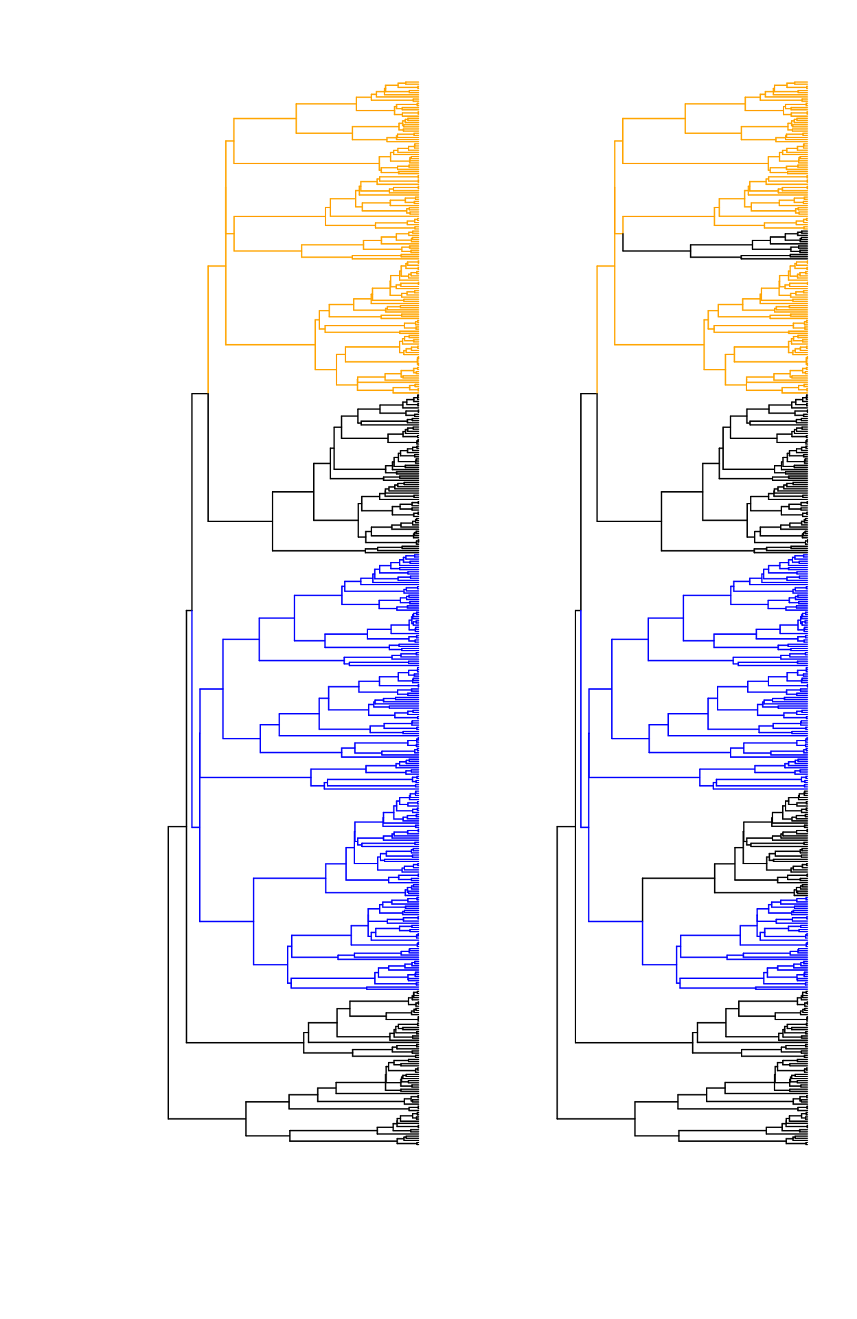
The edges are painted by regime, assuming an optimum for each color. As shown in Ho and Ane (2014a) the left shows an case of unidentifiability case because every regime forms a connected component. The tree on the right shows a case of identifiability because the black regime covers two completely disconnected parts in the tree.
Using the trees in Figure 1, we can conduct a formal test of identifiability of the parameters in the model. Let’s try the unidentifiable case:
load("simUnidentifiable.Rsave")
check.identify(phy, data)
## The regime optima are unidentifiable.## [1] 0Now, the identifiable case:
load("simIdentifiable.Rsave")
check.identify(phy, data)
## The regime optima are identifiable.## [1] 1Another way to diagnose identifiability is to look at the
$regime.weights now provided as part of the model fit
output. If the weights for every taxon in a given regime are identical,
then the expected values of any two taxa in this regime are also
identical. This was shown in the mathematical proof of Ho and Ane
(2014a, see Appendix 1). It is important to note that we have seen in
simulation that even the unidentifiable cases perform well. However,
this may be illusory, and we recommend this test always be used as a
guide, especially in instances where the resulting model fit is unstable
or seems off.
Contour plots
Confidence intervals are typically estimated for each parameter individually. However, the confidence intervals calculated for pairs of correlated parameters can be much wider than their respective univariate confidence intervals. For example, for OU models a decrease in has a similar effect as an increase in : less variation at the tips. There are differences, of course, so the parameters are identifiable (greater tends to erase phylogenetic signal, whereas lower does not). For practical problems, it is possible to have a ridge of nearly equal likelihood where if you change just one parameter, this is enough to move it off the ridge, but if you were to change both this would result in simply sliding along the ridge. This “ridge” behavior is precisely what happens when the is included in the model.
We now allow users to create contour maps of the likelihood surface
for any pair of parameters in a given OUwie model.
Specifically, we sample a large set of points using a latin hypercube
design, and one by one we use these as fixed values for our focal
parameters, and we then search for the maximum likelihood estimates for
the remaining parameters in the model. This step is done using the new
OUwie.contour() function. We will use the trees from above,
to show what a “ridge” looks likes.
load("simsOUidentify_8")
surfaceDatThetaR_2 <- OUwie.contour(oum.root, focal.params = c("theta_Root",
    "theta_2"), focal.params.upper = c(10, 10), nreps = 1000, n.cores = 4)
surfaceDatTheta1_2 <- OUwie.contour(oum.root, focal.params = c("theta_1", "theta_2"),
    focal.params.upper = c(10, 10), nreps = 1000, n.cores = 4)
We want to look at the likelihood surface for
vs.
and for
vs. ,
for an OUM model with the
included in the model. The pair of parameters to examine is passed by
focal.param, and the parameters need to be either “theta”,
“alpha”, or “sigma.sq”. For example, to look at sigma.sq from the first
regime and alpha from the second regime, one would pass
focal.param = c( "sigma.sq_1", "alpha_2"). If the regimes
are input as characters like, say, flower color, the focal parameter
would be focal.param = c( "sigma.sq_Red", "sigma.sq_Blue").
Note that the OUwie.contour function can also be used
across multiple processors (n.cores!=NULL). Once the set of
points have been evaluated, the plot of the likelihood surface can be
generated by inputting OUwie.contour into a plotting
function:
plot(surfaceDatThetaR_2, mle.point = "red", levels = c(0:20 * 0.1), xlab = expression(theta[root]),
    ylab = expression(theta[2]), xlim = c(0, 5, 1), ylim = c(0, 5, 1), col = grey.colors(21,
        start = 0, end = 1))
A few notes about the inputs for the plotting function. First, it
requires an object of class OUwie.contour. Second, by
default mle.point=NULL, which means the MLE point on the
surface will not be plotted, unlesss a color is specified. The axis
labels can be customized, or left as NULL, in which case the focal.param
input from the OUwie.contour function will be used. The
limits to both the x and y axes (the first two values), as well as the
spacing (the third value) can be also specified. Finally, the levels and
the color vector must be of the same length. In the example above, the
levels correspond to the space within 2 log-likelihood from the MLE,
with colors increasingly becoming lighter as the distance from the MLE
increases.
Using a simulated data set, Figure 2 shows the impact of including the into the model – that is, the likelihood surface forms a ridge where linear combinations of parameter values produce identical likelihoods. In such situations the MLE is undefined and the parameters are generally unidentifiable. When the is dropped from the model, as shown in Figure 3, MLE estimates of , , are sufficiently peaked and are clearly separately identifiable.
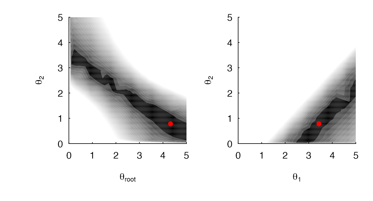
A contour plot of a OUM model, with the included in the model. (A) The contour for when and are specified as the focal parameters, and (B) shows the likelihood surface for when and are specified. In both cases, the likelihood surface appears as a ridge, indicating that the regimes are not separately identifiable.
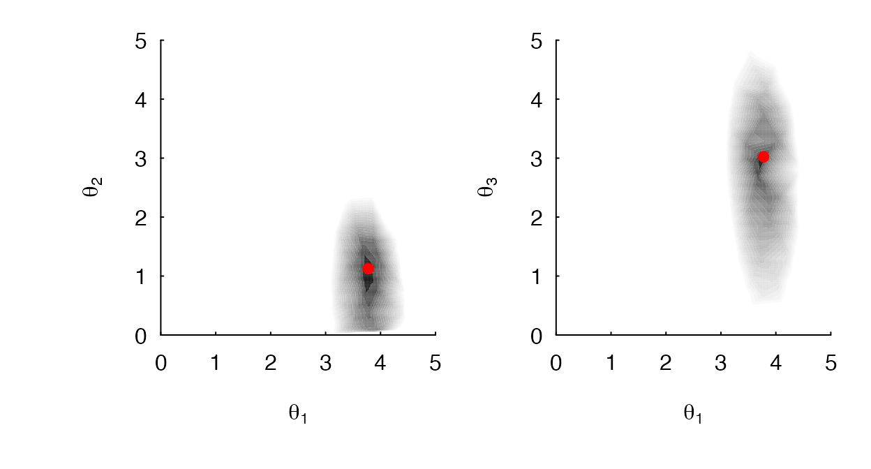
A contour plot of a OUM model, with the removed from the model. (A) The contour for when and are specified as the focal parameters, and (B) for when and are specified, the likelihood surface is sufficiently peaked. In other words, the likelihood surface no longer appears as a ridge and regimes are separately identifiable.
Ancestral trait reconstruction
Since OUwie was first released we’ve received a deluge
of requests to allow for ancestral trait reconstruction. One such
request made its way onto the public R-SIG-PHYLO discussion forum, which
stimulated an important conversation about not whether or not you
could estimate ancestral states, but, rather, should
you. The answer is “it’s complicated” and we honestly don’t recommend
it. In our view, the intended use case is just to visualize what the
model is saying about evolution to help intuition. For example, is the
model something you can believe in? But, if you don’t want to listen to
us regarding the merits of ancestral trait reconstructions, here is a
sample of comments from other experts in the field:
So in short, yes, you can do it, with any number of methods. But why? If you can answer your biological question with methods that do not involve estimation of a parameter that is inherently fraught with error, it might be better to go another way. Bottom line - use caution and be thoughtful! – Marguerite Butler
I would add an extra caveat to Marguerite’s excellent post: Most researchers work with extant taxa only, ignoring extinction. This causes a massive ascertainment bias, and the character states of the extinct taxa can often be very different to the ancestral state reconstructions, particularly if the evolutionary model is wrong. E.g. there has been an evolutionary trend for example. Ancestral state reconstructions based only on extant taxa should be treated as hypotheses to be tested with fossil data. I wouldn’t rely on them for much more. – Simone Blomberg
While I am at it, let me echo Simone and Marguerite’s warnings. The predicted ancestral states will reflect the process you assumed to predict them. Hence, if you use them to make inferences about evolution, you will recover your own assumptions. I.e. if you predict from a model with no trend, you will find no trend, etc. Many comparative studies are flawed for this reason. – Thomas Hansen
Let me add more warnings to Marguerite and Thomas’s excellent responses. People may be tempted to infer ancestral states and then treat those inferences as data (and also to infer ancestral environments and then treat those inferences as data). In fact, I wonder whether that is not the main use people make of these inferences. But not only are those inferences very noisy, they are correlated with each other. So if you infer the ancestral state for the clade (Old World Monkeys, Apes) and also the ancestral state for the clade (New World Monkeys, (Old World Monkeys, Apes)) the two will typically not only be error-prone, but will also typically be subject to strongly correlated errors. Using them as data for further inferences is very dubious. It is better to figure out what your hypothesis is and then test it on the data from the tips of the tree, without the intermediate step of taking ancestral state inferences as observations. The popular science press in particular demands a fly-on-the-wall account of what happened in evolution, and giving them the ancestral state inferences as if they were known precisely is a mistake. – Joe Felsenstein
The minor twist I would throw in is that it’s difficult to make universal generalizations about the quality of ancestral state estimation. If one is interested in the ancestral state value at node N, it might be reasonably estimated if it is nested high up within the phylogeny, if the rates of change aren’t high, etc. And (local) trends etc might well be reliably inferred. We are pretty confident that the common ancestor of humans and chimps was larger than many deeper primate ancestors, for instance. If N is the root of your available phylogeny, however, you have to be much more cautious. – Nick Matzke
I’ll also add that I think there’s a great deal to be skeptical of ancestral trait reconstruction even when large amounts of fossil data is available. You can try the exercise yourself: simulate pure BM on a non-ultrametric tree with lots of ‘extinct’ tips, and you’ll still find pretty large confidence intervals on the estimates of the trait values. What does it mean to do ancestral trait reconstruction, if our calculations of uncertainty are that broad? – Dave Bapst
These people probably know better than anyone about the power and limitations of the OU model in phylogenetics. So, don’t listen to us, listen to them!
Still determined? Ok, fair enough. It is straightforward to run the
ancestral trait reconstruction in OUwie. All you need is an
object of class OUwie, which is plugged directly into the
new OUwie.anc() function:
data(tworegime)
set.seed(42)
ouwiefit <- OUwie(tree, trait, model = "OUM", scaleHeight = TRUE, root.station = FALSE,
    shift.point = 0.5, algorithm = "invert", quiet = TRUE, check.identify = FALSE)
recon <- OUwie.anc(ouwiefit)Ah! If you run the code above a somewhat snarky response is printed
to the screen. Since you are here reading this, we think this is
sufficient, and you are at least aware that we are not huge fans of this
approach. So, there is no need to read the manual (it’s basically the
same as what you see here), and the proper way to call the
OUwie.anc() function call is simply add in
knowledge=TRUE:
recon <- OUwie.anc(ouwiefit, knowledge = TRUE)## [1] "Doing reconstructions"
## Working on node 1 of 62 Working on node 2 of 62 Working on node 3 of 62 Working on node 4 of 62 Working on node 5 of 62 Working on node 6 of 62 Working on node 7 of 62 Working on node 8 of 62 Working on node 9 of 62 Working on node 10 of 62 Working on node 11 of 62 Working on node 12 of 62 Working on node 13 of 62 Working on node 14 of 62 Working on node 15 of 62 Working on node 16 of 62 Working on node 17 of 62 Working on node 18 of 62 Working on node 19 of 62 Working on node 20 of 62 Working on node 21 of 62 Working on node 22 of 62 Working on node 23 of 62 Working on node 24 of 62 Working on node 25 of 62 Working on node 26 of 62 Working on node 27 of 62 Working on node 28 of 62 Working on node 29 of 62 Working on node 30 of 62 Working on node 31 of 62 Working on node 32 of 62 Working on node 33 of 62 Working on node 34 of 62 Working on node 35 of 62 Working on node 36 of 62 Working on node 37 of 62 Working on node 38 of 62 Working on node 39 of 62 Working on node 40 of 62 Working on node 41 of 62 Working on node 42 of 62 Working on node 43 of 62 Working on node 44 of 62 Working on node 45 of 62 Working on node 46 of 62 Working on node 47 of 62 Working on node 48 of 62 Working on node 49 of 62 Working on node 50 of 62 Working on node 51 of 62 Working on node 52 of 62 Working on node 53 of 62 Working on node 54 of 62 Working on node 55 of 62 Working on node 56 of 62 Working on node 57 of 62 Working on node 58 of 62 Working on node 59 of 62 Working on node 60 of 62 Working on node 61 of 62 Working on node 62 of 62 [1] "Done reconstructions"From there, you can then easily plot these reconstructions using an
internal function that recognizes the OUwie and
OUwie.anc class:
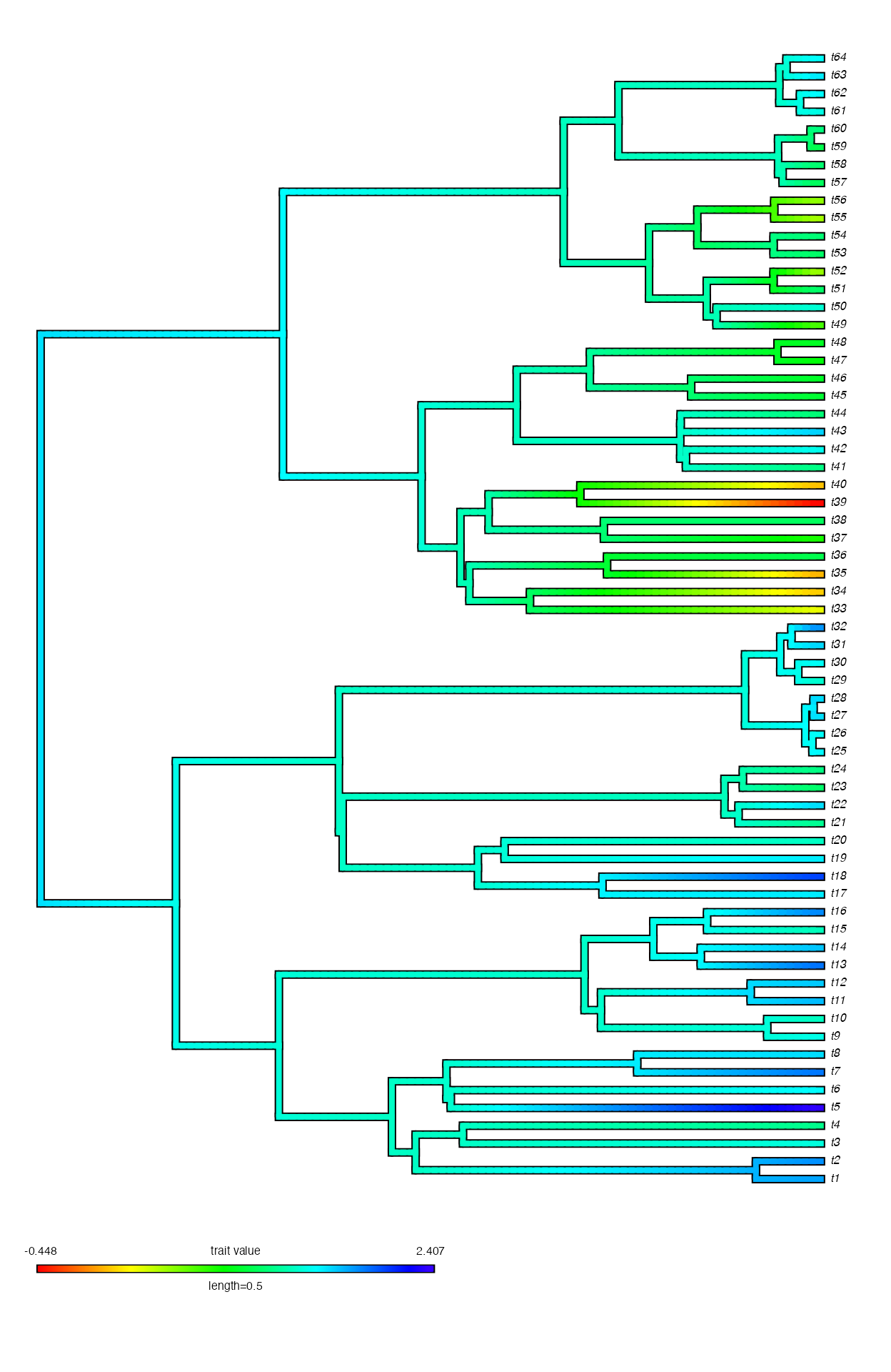
A plot of the ancestral state reconstruction under an OUwie model.
Generalized three-point structured algorithm
A long time complaint about OUwie is that it does not
scale well when trees exceed 1000 species. This was largely due to the
fact that we relied completely on linear algebra functions, in
particular, computing the determinant of the variance-covariance matrix,
,
as well as inverting it to obtain the log-likelihood and calculate
.
Starting with OUwie version 2.5, we include the generalize
three-point algorithm of Ho and Ane (2014b) that bypasses the need for
these inefficient calculations. The details of this algorithm are beyond
the scope of this vignette and readers should consult Ho and Ane
(2014b). The generalized three-point structured algorithm can now be
specified in the OUwie() function call:
data(tworegime)
three.point <- OUwie(tree, trait, model = "OUMV", root.station = FALSE, scaleHeight = TRUE,
    shift.point = 0.5, algorithm = "three.point", quiet = TRUE, check.identify = FALSE)
three.point
##
## Fit
## lnL AIC AICc BIC model ntax
## -14.79505 39.59011 40.62459 50.38453 OUMV 64
##
##
## Rates
## 1 2
## alpha 1.7124628 1.712463
## sigma.sq 0.3518159 1.076873
##
## Optima
## 1 2
## estimate 1.676914 0.5567907
## se NA NA
##
##
## Half life (another way of reporting alpha)
## 1 2
## 0.4047663 0.4047663
##
## Arrived at a reliable solutionWe can compare this to the using the standard matrix determinant and matrix inversion:
data(tworegime)
invert <- OUwie(tree, trait, model = "OUMV", root.station = FALSE, scaleHeight = TRUE,
    shift.point = 0.5, algorithm = "invert", quiet = TRUE)
## Warning: The supplied regime painting may be unidentifiable for the regime
## painting. All regimes form connected subtrees.
invert##
## Fit
## lnL AIC AICc BIC model ntax
## -14.79506 39.59011 40.6246 50.38453 OUMV 64
##
##
## Rates
## 1 2
## alpha 1.7110818 1.711082
## sigma.sq 0.3517019 1.076479
##
## Optima
## 1 2
## estimate 1.676894 0.5563541
## se 0.112031 0.3020699
##
##
## Half life (another way of reporting alpha)
## 1 2
## 0.405093 0.405093
##
## Arrived at a reliable solutionIn this particular example, the log-likelihoods are identical.
However, users are cautioned that some slight differences between the
algorithm="invert" and algorithm="three.point"
will likely be common. The use of the three-point structured algorithm
requires that
be optimized like any other parameter in the model, whereas with the
matrix inversion approach
are solved numerically. This means that when there are differences in
the log-likelihood it is likely because one or more of
is not at the MLE after using the three-point algorithm. Users are
encouraged then to examine the contours of pairs of
.
Also note, that the speed-ups afforded by the three-point algorithm is
most observable when the tree size exceeds 500 taxa.
Estimating tip fog
In comparative biology, we often overlook the complexity of uncertainty. We might consider “measurement error” as the standard error of the observed measurements for species, but the common default is to assume this error is zero. Moreover, the array of factors contributing to this uncertainty extends far beyond what we traditionally categorize as measurement error. This intraspecific variance has been described by various terms, including “specific variances”, “residual variation”, “phenotypic variation”, and measurement error. Some of these terms suggest specific mechanisms. Other terms are more descriptive but may have meanings outside the field that can cause confusion. To avoid ambiguity, we recently propose a new term: “tip fog” (Beaulieu and O’Meara, 2024), This term captures the variance that occurs at the present between the true species mean derived from the evolutionary process and what an experimenter records as a value, without being tied to any particular mechanism, and it applies to characters that are discrete or continuous.
There are various ways to specify tip fog. First, recall from the
individual manuals that the trait data.frame must have column entries in
the following order: species names, current selective regime, and the
continuous trait of interest. If the user wants to incorporate tip fog
based on their own measurements (tip.fog="known"), then a
fourth column must be included that provides the standard error
estimates for each species mean. However, a global tip fog for all
taxa can be estimated from the data (tip.fog="estimate").
Specifically, to estimate the tip fog parameter:
data(tworegime)
invert <- OUwie(tree, trait, model = "OUMV", root.station = FALSE, scaleHeight = TRUE,
    shift.point = 0.5, tip.fog = "estimate", algorithm = "invert", quiet = TRUE)
invert
In simulation we’ve found that not accounting for tip fog can have a
substantial effect on the rate estimates. That is, rates quicky become
severally overestimated with even a modest amount of tip fog. It is for
these reasons we suggest that user at least set
tip.fog="estimate" for now. In future version, this option
will become the default.
References
Beaulieu J.M., D.C. Jhwueng, C. Boettiger, and B.C. O’Meara. 2012. Modeling stabilizing selection: Expanding the Ornstein-Uhlenbeck model of adaptive evolution. Evolution, 66:2369-2383.
Butler M.A., A.A. King A.A. 2004. Phylogenetic comparative analysis: A modeling approach for adaptive evolution. American Naturalist, 164:683-695.
Ho, L.S.T., and C. Ane. 2013. Asymptotic theory with hierarchical autocorrelation: Orstein-Uhlenbeck tree models. The Annals of Statistics, 41:957-981.
Ho, L.S.T., and C. Ane. 2014a. Intrinsic inference difficulties for trait evolution with Ornstein-Uhlenbeck models. Methods in Ecology and Evolution, 5: 1133-1146.
Ho, L.S.T., and C. Ane. 2014b. A linear-time algorithm for Gaussian and non-Gaussian trait evolution models. Systematic Biology, 63:397-408.